How Much Contango in Gold Futures?

by BullionRadar

Gold is one of the world’s oldest and most actively traded commodities, and its futures contract on COMEX (symbol GC) is the benchmark for pricing and hedging in the bullion business. Whether you’re a refiner, a wholesaler, or an institutional investor, GC futures are the main tool for managing exposure to physical gold.

The slope of the gold futures curve, whether in contango (later contracts more expensive than near ones) or backwardation (later contracts cheaper), matters for several reasons. Contango represents the cost of carry: financing, storage, and insurance. Backwardation, although rare for gold, can signal tight physical supply or unusual demand for immediate delivery. Understanding the historical size of that contango helps traders gauge hedging costs and recognize market stress when spreads deviate from expectations.

Methodology

To get a quantitative picture, we pulled daily GC futures data from 2010 onward using Databento. The goal was to measure the annualized return from rolling from the nearest active contract into the next one, essentially the cost (or benefit) of maintaining a long futures position over time.


import pandas as pd
from datetime import datetime
import calendar

MOIS_CODES = {'F': 1, 'G': 2, 'H': 3, 'J': 4, 'K': 5, 'M': 6,
              'N': 7, 'Q': 8, 'U': 9, 'V': 10, 'X': 11, 'Z': 12}

def parse_expiration(symbol: str, event_year: int):
    if not symbol or len(symbol) < 2 or '-' in symbol:
        return None
    month = MOIS_CODES.get(symbol[-2])
    if not month:
        return None
    try:
        year_code = int(symbol[-1])
        possible_years = [2000 + year_code, 2010 + year_code, 2020 + year_code, 2030 + year_code]
        year = min(possible_years, key=lambda y: abs(y - event_year))
        last_day = calendar.monthrange(year, month)[1]
        return datetime(year, month, last_day).date()
    except ValueError:
        return None

def aggregate_top2(group: pd.DataFrame) -> pd.Series:
    if len(group) < 2:
        row = group.iloc[0]
        return pd.Series({
            'near_symbol': row['symbol'],
            'far_symbol': None,
            'near_expiration': row['expiration_date'],
            'far_expiration': None,
            'near_close': row['close'],
            'far_close': None,
            'near_volume': row['volume'],
            'far_volume': None,
            'diff_days': None,
            'annualized_return': None
        })
    near, far = group.iloc[0], group.iloc[1]
    diff_days = (far['expiration_date'] - near['expiration_date']).days
    annualized_return = ((far['close'] - near['close']) / near['close']) / diff_days * 365 if diff_days > 0 else None
    return pd.Series({
        'near_symbol': near['symbol'],
        'far_symbol': far['symbol'],
        'near_expiration': near['expiration_date'],
        'far_expiration': far['expiration_date'],
        'near_close': near['close'],
        'far_close': far['close'],
        'near_volume': near['volume'],
        'far_volume': far['volume'],
        'diff_days': diff_days,
        'annualized_return': annualized_return
    })

df = pd.read_csv("GC.csv", sep=",")
df.columns = df.columns.str.strip()
df = df[~df['symbol'].str.contains('-')]
df['ts_event'] = pd.to_datetime(df['ts_event']).dt.date
df['expiration_date'] = df.apply(lambda row: parse_expiration(row['symbol'], row['ts_event'].year), axis=1)

df_top2 = (
    df.sort_values(['ts_event', 'volume'], ascending=[True, False])
      .groupby('ts_event')
      .head(2)
      .sort_values(['ts_event', 'expiration_date'])
)

df_daily = (
    df_top2.groupby('ts_event')[['symbol','expiration_date','close','volume']]
           .apply(aggregate_top2)
           .reset_index()
)

print(df_daily.head())
df_daily.to_csv("result2.csv", index=False)

The updated Python workflow did three main things:

  1. Parsed contract expirations : Each GC symbol encodes its month and year (e.g., “GCZ3” = December 2023). The code mapped month codes to actual months and guessed the correct year based on the trade date.

  2. Identified the top two contracts by volume per day : This filters out illiquid contracts and spreads, leaving the two front-month contracts that represent the live curve.

  3. Computed the daily roll yield : For each trading day, it calculated the price difference between the near and next contract, adjusted for the number of days between expirations, and annualized the result. The daily series was then averaged by month to smooth noise.

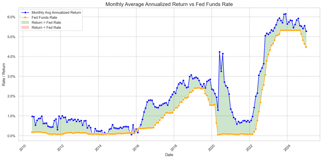
Finally, these monthly average annualized returns were plotted against the Federal Funds rate, the baseline cost of financing in U.S. dollars. Comparing them shows whether gold’s contango aligns with funding costs or diverges due to market-specific factors.

Results and Interpretation

The resulting chart shows two lines: the blue line is the monthly average annualized roll return (contango/backwardation), and the orange line is the Fed Funds rate. The shaded areas highlight when gold’s contango was greater than (green) or less than (red) the Fed rate.

For most of the period, the two lines track each other well, evidence that the cost of carry in gold broadly mirrors money market rates. But there are two notable exceptions:

  • The extraordinary widening in 2020: At the onset of COVID-19, physical bullion flows broke down. Refiners in Switzerland shut down, international flights were grounded, and gold couldn’t easily reach COMEX delivery points. Liquidity stress and margin calls caused futures prices to detach, creating a historic surge in contango. This wasn’t a data error, it’s a known event where futures spreads blew out for several months.

  • The flat curve of 2014–2016: In contrast, some periods during these years show contango dipping below the Fed Funds rate. With ultra-low rates and weak gold lease demand, carry returns compressed. It wasn’t dramatic, but it’s a reminder that the curve can sometimes underperform funding benchmarks even in calm markets.

These episodes illustrate that while contango in gold is usually small and predictable, extraordinary circumstances, whether a global pandemic or extreme monetary policy, can disrupt the pattern.

Conclusion

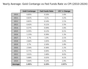
Over more than a decade of history, GC futures have generally shown a steady, modest contango aligned with U.S. interest rates. For the bullion industry, this offers a useful reference: rolling gold futures typically costs about the prevailing short-term funding rate, plus minor adjustments for storage and insurance.

Yet, the 2020 spike demonstrates how quickly that equilibrium can break when physical logistics or liquidity are strained. And the quieter 2014–2016 flattening shows that even without drama, shifts in rates and lease demand can move the curve away from expectations.

For traders, refiners, and investors, the key takeaway is that contango isn’t a fixed number, it’s a reflection of both financing conditions and market health. Tracking these spreads over time doesn’t just tell you about hedging costs; it can also serve as an early warning signal of stress, or an opportunity, in the gold market.

You may also like